The steppingstone method is used to estimate the marginal likelihood of a model. The measures the average fit of the model to the data, and is a popular way of comparing models in Bayesian analyses. This tutorial implements the simpler version of the steppingstone method described by Xie et al. (2011). Generalized steppingstone (Fan et al. 2011) is much more efficient computationally, so you may want to implement that as a challenge after implementing the Xie et al. (2011) version.
What is the marginal likelihood?
The marginal likelihood is the denominator in Bayes’ Rule.
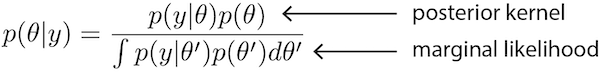 It serves as the normalizing constant that ensures that posterior probabilities sum to 1.0 over all possible parameter combinations, but it can also be interpreted as the weighted average likelihood where the weights are provided by the joint prior distribution. Because the likelihood measures fit of the model to the data, we can think of the marginal likelihood as the average fit of the model to the data. Bayesian model selection based on marginal likelihood is thus concerned with finding the model that fits the data best on average across all of parameter space. Because all parameters of the model are integrated out in computing the marginal likelihood, the marginal likelihood can be used to compare models with differing dimensions on the same data.
The Bayes Factor is the ratio of marginal likelihoods from two competing models. If the Bayes Factor is 1, it means both models fit the data equally well on average. Bayes Factors less than 1 mean that the model in the denominator fits the data better (on average), while a Bayes Factor greater than 1 means that it is the model on top (in the numerator) that is the better fitting model. Take care to distinguish the Bayes Factor, which is a ratio of two marginal likelihoods, from the log Bayes Factor, which is the natural logarithm of the Bayes Factor. The log Bayes Factor is the difference between two log marginal likelihoods and is what is normally reported because marginal likelihoods are usually computed on the log scale. When you are comparing Bayes Factors to commonly-cited rules of thumb to determine how much significance to attribute to them, be sure that your rule of thumb is on the same scale as your Bayes Factor: that is, don’t judge a Bayes Factor by a rule of thumb written for log Bayes Factors, or vice versa!
How steppingstone works
In its role as normalizing constant, the marginal likelihood has a graphical interpretation that makes understanding the steppingstone method for estimating the marginal likelihood much easier. Consider the following binomial experiment: you flip a coin 3 times and see 1 head. The likelihood is the binomial probability of seeing 1 head out of 3 flips when the underlying probability of a head on any given flip is p. Let’s assume a Uniform(0,1) distribution for p, which is completely agnostic about the value of p: for example, it says that the chances that our coin is perfectly fair is the same as the chances that it is a trick coin that always comes up heads. While we might argue that such a prior is not very reasonable, this prior has the benefit of being very simple. The prior density is simply 1 for every possible value of p. The figure below shows a plot of both the prior (the straight line at the top) as well as the posterior kernel, which is the unnormalized posterior density. Note that the posterior kernel is entirely beneath the prior density: the area under the posterior kernel is thus smaller than the area under the prior density, which is 1 because the area under the prior is a perfect square with height 1 (because the density is 1 everywhere) and width 1 (because the support of p, i.e. the region of parameter space in which p has non-zero probability density, is the interval [0,1]). This nesting of the posterior kernel within the prior will always be the case if the data are discrete (true for both coin flipping experiments and nucleotide sequences) because, in the case of discrete data, the likelihood is a probability (not a probability density) and thus its value must be less than or equal to 1. Because the posterior kernel is the likelihood multiplied by the prior, that means that the posterior kernel must be less than or equal to the prior density. Our goal is to estimate the area under the posterior kernel: that area equals the marginal likelihood because it is the integral, over the entire parameter space, of the likelihood times the prior, which is exactly what is shown in the equation above.
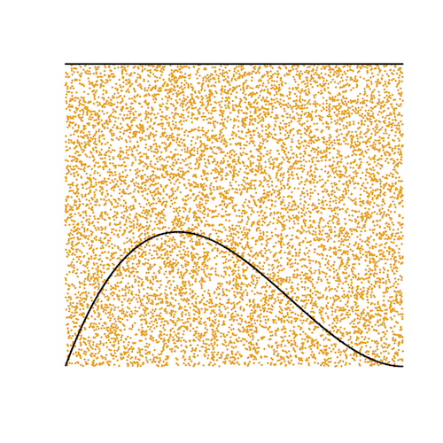 You can see that one way to estimate the area under the posterior kernel would be to (figuratively) throw darts (the orange dots) at the square representing the prior (which has area 1) and determine the fraction of those darts that also fall underneath the posterior kernel. If you understand that, then you already understand the steppingstone method! In this case, the true marginal likelihood is 0.25 and, of the 10,000 darts thrown, 2501 landed beneath the line representing the posterior kernel, so our estimated marginal likelihood is 0.2501. Not bad!
Reality rears its ugly head
In practice, the estimation of the marginal likelihood is complicated by the fact that the posterior kernel normally has a really tiny area compared to the area under the prior density. Remember that the posterior kernel is unnormalized: once we have the marginal likelihood value, we could normalize the posterior kernal by dividing every value by the marginal likelihood (normalizing constant) to yield a proper posterior distribution that, like the prior, integrates to 1.
What if, instead of flipping the coin just 3 times, we instead flipped it 40,000 times and happened to record 20,000 heads. We now have much more data, which makes the area under the posterior kernel much smaller.
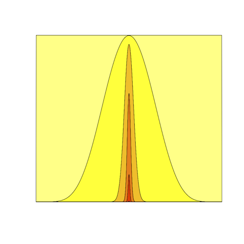 In this image, there are 6 lines plotted. The 1st one (straight line) is, again, the flat Uniform(0,1) prior and is hidden because it is coincident with the line across the top of the plot. The 6th line plotted is a very tiny nubbin - you may need to zoom in to even see it. That nubbin is the posterior kernel. Hopefully you can begin to see the problem. If we throw darts at the square prior area, chances are that very few (perhaps zero) of them will land underneath that nubbin, so, unless we throw an very large number of darts, we may estimate the marginal likelihood to be zero, which is clearly the wrong answer. The problem is not with our method, it is with the efficiency of our method. It would be great to have a way to get the area under the nubbin without having to throw an astronomical number of darts.
The steppingstone method, as the name suggest, breaks up the problem into smaller pieces, each of which is easier to estimate, just as steppingstones placed at regular intervals in a stream help you cross the stream without getting your feet wet. We define a series of power posterior distributions that form a series of nested densities, each enclosing the next. Throwing darts at the 1st (the prior) allows us to estimate the area under the 2nd. Throwing darts at the 2nd allows us to estimate the area under the 3rd, and so on. Because the (i+1)st distribution is not that much smaller than the ith distribution, each of these estimates can be done efficiently and with arbitrary accuracy.
The power posterior distribution is defined as the product of the prior density and the likelihood raised to a power β that is in the interval [0,1].
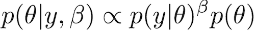 If β equals 0, then the likelihood disappears because any number raised to the power 0 is just 1. Thus, the power posterior kernel when β is set to 0 is just the prior distribution. If β is set to 1, then the power posterior kernel equals the posterior kernel. Any value of β in between 0 and 1, however, yields a distribution intermediate between the prior and the posterior kernel. Xie et al. (2011) found that choosing βs such that most of them were near the prior was better than spacing them evenly between 0 and 1. I’ll show you how to do that when describing the code, but we’ll introduce a setting
 ssalpha that determines how much of a prior bias there is to the choice of β values: a smaller value of ssalpha means more clumping of βs near the prior, and values of ssalpha near 0.2 or 0.3 work well.
Putting it all together
Because our program can already run multiple chains with different heating powers, it is very tempting to just assign a different power posterior to each heated chain, and that is in fact how we will implement the steppingstone method. The _heating_power of each heated chain will equal one of the β values from the series we’ve decided upon. We do not need to assign β = 1 (the power representing the posterior kernel) to any heated chain because (oddly) we do not need samples from the posterior kernel to carry out the steppingstone method. We always (metaphorically) throw darts only at the larger of the two areas we are comparing, so the last power posterior we need to sample is the one that just encloses the posterior kernel. Once we have samples from each power posterior in the series, we can estimate a ratio of areas from each. If we represent the areas under each of the power posteriors as a series of letters, with a being the area under the posterior kernel and f being the area under the prior, note that the product of all these ratios equals the marginal likelihood due to the cancellation of all terms except the marginal likelihood (a) and prior (f).
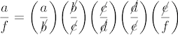 Remember that the prior has area one, so f equals 1 and thus this final ratio really just equals the area under the posterior kernel, a. Pretty cool, eh?
| Step | Title | Description |
| Step 20.1 | Adding settings for steppingstone | Modifying the Strom class to add settings for steppingstone. |
| Step 20.2 | Modifying the Chain class for steppingstone | Modifying the Chain class for steppingstone. |
| Step 20.3 | Updating the Updater | Here we add a data member and member function to inform Updater that only the likelihood should be heated |
| Step 20.4 | Test steppingstone | Test the steppingstone method |
Literature Cited
Xie, W., P. O. Lewis, Y. Fan, L. Kuo, and M.-H. Chen. 2011. Improving marginal likelihood estimation for Bayesian phylogenetic model selection. Systematic Biology 60:150-160. DOI:10.1093/sysbio/syq085
Fan, Y., R. Wu, M.-H. Chen, L. Kuo, and P. O. Lewis. 2011. Choosing among partition models in Bayesian phylogenetics. Molecular Biology and Evolution 28:523-532. DOI:10.1093/molbev/msq224